


近邻算法(k-Nearest Neighbor)是CS231n课程介绍的第一个算法,此算法和神经网络没有任何关系,实际中也极少使用,但学习使用KNN算法可以获得对图像分类方法的基本认知。
先决条件
在开始写作业前,你需要做一些准备工作。
Jupyter Notebook先决条件
你可以在这里下载官方提供的CS231n Assignment1的 Jupyter笔记本。
在Anaconda Prompt Powershell中输入conda activate cs231,接着cd到assignment1目录下,输入jupyter notebook开启Ipython笔记本,打开knn.ipynb即可开始本次作业。
在开始之前,需要注意,由于Jupyter Notebook的某种bug,CIFAR-10的路径变量cifar10_dir需要赋值为绝对路径,同时在路径前加上r来忽略转义,像下面这样:
# Load the raw CIFAR-10 data.
cifar10_dir = r'D:\Users\VonBrank\Documents\GitHub\code-learning\algorithm\deep-learning\computer-visualization\cs231n\datasets\cifar-10-batches-py'
到此为止,写代码前的准备工作就完成了。
Numpy先决条件
Numpy是CS231n课程中所需的科学计算库,其优秀的矩阵运算性能对图像处理有巨大帮助,在此介绍KNN算法中需使用的Numpy函数。
基于元素的运算
Numpy的所有计算都是基于元素的。设
A、B是两个矩阵,则A + B表示两个矩阵的对应位相乘,A × B同理;而若要作矩阵乘法,让B右乘A,则可以写成A.dot(B)或A @ B。Numpy数组切片
Numpy幂运算
np.sum()np.sqrt()np.argsort()np.argmax()np.bincount()
KNN算法
思路
KNN算法遵循以下步骤:
取CIFAR-10数据集中的一张图片 ,将其拉伸为一个3072维的向量,训练集中的每个向量都可以视作 维欧氏空间中的一个点。
对测试集中的每一张图片作相同的操作,计算其与训练集中每一张图的欧式距离。
对测试集中的任意一张图片,考察其在训练集中的前 近的点(用 距离计算),分类数最大的分类即预测为此图像的所属分类。
为了便于理解,我们将 维的空间简化为 维空间,在理解了二维空间的KNN算法后,扩展至 维甚至更多维数的KNN将变得更易于理解。
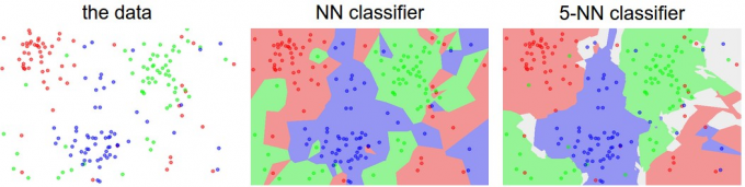
如上图所示,若将图像映射为二维平面上的一个点,可以看出,若使用KNN算法遍历空间中的所有点,可将二维空间划分为若干区域,每个区域表示一个分类。
对于 的情况,即NN(Nearest Neighbor)算法,可看出,对于空间中任意一点,将离其最近的训练集中的点所属分类判定为该点所属的分类。
对于 的情况,即KNN算法的一般情况。举例来说,假设对于一个点,离该点前 近的训练集中的点中,属于 红色 分类的点是最多的,即可将该点所属的分类判定为 红色 分类。
需要说明的是,定义两个点,即两个图像之间的距离,通常使用 距离,即欧几里得距离,计算方法如下:
为了实现这个算法,knn.ipynb将指示我们从两重循环到一重循环,再到以纯向量化代码实现 距离的计算,并体验其优化过程。
实现
由于之后每个task的流程都差不多,文本将展示一个完整的流程,之后的记录不再赘述。虽然CS231n官方在笔记本里提供的大量轮子,只要求我们编写核心代码,但仍推荐阅读这些轮子的实现。
初始化
In[1]
# Run some setup code for this notebook.

import random
import numpy as np
from cs231n.data_utils import load_CIFAR10
import matplotlib.pyplot as plt

# This is a bit of magic to make matplotlib figures appear inline in the notebook
# rather than in a new window.
%matplotlib inline
plt.rcParams['figure.figsize'] = (10.0, 8.0) # set default size of plots
plt.rcParams['image.interpolation'] = 'nearest'
plt.rcParams['image.cmap'] = 'gray'

# Some more magic so that the notebook will reload external python modules;
# see http://stackoverflow.com/questions/1907993/autoreload-of-modules-in-ipython
%load_ext autoreload
%autoreload 2
加载数据
In[2]
# Load the raw CIFAR-10 data.
cifar10_dir = r'D:\Users\VonBrank\Documents\GitHub\code-learning\algorithm\deep-learning\computer-visualization\cs231n\datasets\cifar-10-batches-py'

# Cleaning up variables to prevent loading data multiple times (which may cause memory issue)
try:
   del X_train, y_train
   del X_test, y_test
   print('Clear previously loaded data.')
except:
   pass

X_train, y_train, X_test, y_test = load_CIFAR10(cifar10_dir)

# As a sanity check, we print out the size of the training and test data.
print('Training data shape: ', X_train.shape)
print('Training labels shape: ', y_train.shape)
print('Test data shape: ', X_test.shape)
print('Test labels shape: ', y_test.shape)
Out[2]
Training data shape:  (50000, 32, 32, 3)
Training labels shape:  (50000,)
Test data shape:  (10000, 32, 32, 3)
Test labels shape:  (10000,)
预处理数据
随机选取一些图像并输出:
# Visualize some examples from the dataset.
# We show a few examples of training images from each class.
classes = ['plane', 'car', 'bird', 'cat', 'deer', 'dog', 'frog', 'horse', 'ship', 'truck']
num_classes = len(classes)
samples_per_class = 7
for y, cls in enumerate(classes):
    idxs = np.flatnonzero(y_train == y)
    idxs = np.random.choice(idxs, samples_per_class, replace=False)
    for i, idx in enumerate(idxs):
        plt_idx = i * num_classes + y + 1
        plt.subplot(samples_per_class, num_classes, plt_idx)
        plt.imshow(X_train[idx].astype('uint8'))
        plt.axis('off')
        if i == 0:
            plt.title(cls)
plt.show()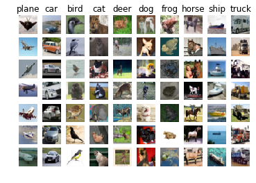
选取CIFAR-10的一个子集进行训练与测试
In[3]
# Subsample the data for more efficient code execution in this exercise
num_training = 5000
mask = list(range(num_training))
X_train = X_train[mask]
y_train = y_train[mask]

num_test = 500
mask = list(range(num_test))
X_test = X_test[mask]
y_test = y_test[mask]

# Reshape the image data into rows
X_train = np.reshape(X_train, (X_train.shape[0], -1))
X_test = np.reshape(X_test, (X_test.shape[0], -1))
print(X_train.shape, X_test.shape)
Out[3]
(5000, 3072) (500, 3072)调用KNN算法
from cs231n.classifiers import KNearestNeighbor

# Create a kNN classifier instance.
# Remember that training a kNN classifier is a noop:
# the Classifier simply remembers the data and does no further processing
classifier = KNearestNeighbor()
classifier.train(X_train, y_train)
两重循环计算 距离
完成cs231n/classifiers/k_nearest_neighbor.py中的compute_distances_two_loops函数:
def compute_distances_two_loops(self, X):
    """
    Compute the distance between each test point in X and each training point
    in self.X_train using a nested loop over both the training data and the
    test data.

    Inputs:
    - X: A numpy array of shape (num_test, D) containing test data.

    Returns:
    - dists: A numpy array of shape (num_test, num_train) where dists[i, j]
      is the Euclidean distance between the ith test point and the jth training
      point.
    """
    num_test = X.shape[0]
    num_train = self.X_train.shape[0]
    dists = np.zeros((num_test, num_train))
    for i in range(num_test):
        for j in range(num_train):
            #####################################################################
            # TODO:                                                             #
            # Compute the l2 distance between the ith test point and the jth    #
            # training point, and store the result in dists[i, j]. You should   #
            # not use a loop over dimension, nor use np.linalg.norm().          #
            #####################################################################
            # *****START OF YOUR CODE (DO NOT DELETE/MODIFY THIS LINE)*****
            dists[i][j] = np.sqrt(np.sum((X[i, :] - self.X_train[j, :]) ** 2))
            pass

            # *****END OF YOUR CODE (DO NOT DELETE/MODIFY THIS LINE)*****
     return dists
验证计算是否正确:
In[4]
# Open cs231n/classifiers/k_nearest_neighbor.py and implement
# compute_distances_two_loops.

# Test your implementation:
dists = classifier.compute_distances_two_loops(X_test)
print(dists.shape)
Out[4]
(500, 5000)可视化结果:
In[5]
# We can visualize the distance matrix: each row is a single test example and
# its distances to training examples
plt.imshow(dists, interpolation='none')
plt.show()
Out[6]
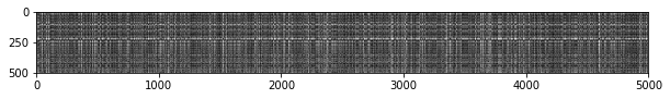
其中,白线意味着对应位置的训练集和测试集相似度非常低。
测试一下:
In[6]
# Now implement the function predict_labels and run the code below:
# We use k = 1 (which is Nearest Neighbor).
y_test_pred = classifier.predict_labels(dists, k=1)

# Compute and print the fraction of correctly predicted examples
num_correct = np.sum(y_test_pred == y_test)
accuracy = float(num_correct) / num_test
print('Got %d / %d correct => accuracy: %f' % (num_correct, num_test, accuracy))
Out[6]
Got 137 / 500 correct => accuracy: 0.274000可以看出, 时,准确率为 。
接着测试 的情况:
In[7]
y_test_pred = classifier.predict_labels(dists, k=5)
num_correct = np.sum(y_test_pred == y_test)
accuracy = float(num_correct) / num_test
print('Got %d / %d correct => accuracy: %f' % (num_correct, num_test, accuracy))
Out[7]
Got 139 / 500 correct => accuracy: 0.278000可以看到, 与 的结果相差不大。
一重循环计算 距离
完成compute_distances_two_loops函数:
def compute_distances_one_loop(self, X):
    """
    Compute the distance between each test point in X and each training point
    in self.X_train using a single loop over the test data.

    Input / Output: Same as compute_distances_two_loops
    """
    num_test = X.shape[0]
    num_train = self.X_train.shape[0]
    dists = np.zeros((num_test, num_train))
    for i in range(num_test):
        #######################################################################
        # TODO:                                                               #
        # Compute the l2 distance between the ith test point and all training #
        # points, and store the result in dists[i, :].                        #
        # Do not use np.linalg.norm().                                        #
        #######################################################################
        # *****START OF YOUR CODE (DO NOT DELETE/MODIFY THIS LINE)*****
        dists[i, :] = np.sqrt(np.sum(((X[i] - self.X_train) ** 2), axis=1))
        # pass

        # *****END OF YOUR CODE (DO NOT DELETE/MODIFY THIS LINE)*****
    return dists
测试一下:
In[8]
# Now lets speed up distance matrix computation by using partial vectorization
# with one loop. Implement the function compute_distances_one_loop and run the
# code below:
dists_one = classifier.compute_distances_one_loop(X_test)

# To ensure that our vectorized implementation is correct, we make sure that it
# agrees with the naive implementation. There are many ways to decide whether
# two matrices are similar; one of the simplest is the Frobenius norm. In case
# you haven't seen it before, the Frobenius norm of two matrices is the square
# root of the squared sum of differences of all elements; in other words, reshape
# the matrices into vectors and compute the Euclidean distance between them.
difference = np.linalg.norm(dists - dists_one, ord='fro')
print('One loop difference was: %f' % (difference, ))
if difference < 0.001:
    print('Good! The distance matrices are the same')
else:
    print('Uh-oh! The distance matrices are different')
Out[8]
One loop difference was: 0.000000
Good! The distance matrices are the same
如果出现上述结果,则证明实现正确。
纯向量化计算 距离
完成compute_distances_no_loops函数:
这里需要将 距离公式展开为多项式,再进行向量化计算。
def compute_distances_no_loops(self, X):
    """
    Compute the distance between each test point in X and each training point
    in self.X_train using no explicit loops.

    Input / Output: Same as compute_distances_two_loops
    """
    num_test = X.shape[0]
    num_train = self.X_train.shape[0]
    dists = np.zeros((num_test, num_train))
    #########################################################################
    # TODO:                                                                 #
    # Compute the l2 distance between all test points and all training      #
    # points without using any explicit loops, and store the result in      #
    # dists.                                                                #
    #                                                                       #
    # You should implement this function using only basic array operations; #
    # in particular you should not use functions from scipy,                #
    # nor use np.linalg.norm().                                             #
    #                                                                       #
    # HINT: Try to formulate the l2 distance using matrix multiplication    #
    #       and two broadcast sums.                                         #
    #########################################################################
    # *****START OF YOUR CODE (DO NOT DELETE/MODIFY THIS LINE)*****

    # 将L2距离展开为多项式,用reshape触发numpy的广播功能
    dists += np.sum(X ** 2, axis=1).reshape(num_test, 1)
    dists += np.sum(self.X_train ** 2, axis=1).reshape(1, num_train)
    dists -= 2 * (X @ self.X_train.T)
    dists = np.sqrt(dists)
    pass

    # *****END OF YOUR CODE (DO NOT DELETE/MODIFY THIS LINE)*****
    return dists
测试一下:
In[9]
# Now implement the fully vectorized version inside compute_distances_no_loops
# and run the code
dists_two = classifier.compute_distances_no_loops(X_test)

# check that the distance matrix agrees with the one we computed before:
difference = np.linalg.norm(dists - dists_two, ord='fro')
print('No loop difference was: %f' % (difference, ))
if difference < 0.001:
    print('Good! The distance matrices are the same')
else:
    print('Uh-oh! The distance matrices are different')
Out[9]
No loop difference was: 0.000000
Good! The distance matrices are the same
如果得出以上结果,则证明实现正确。
比对三种实现方式的速度
In[10]
# Let's compare how fast the implementations are
def time_function(f, *args):
    """
    Call a function f with args and return the time (in seconds) that it took to execute.
    """
    import time
    tic = time.time()
    f(*args)
    toc = time.time()
    return toc - tic

two_loop_time = time_function(classifier.compute_distances_two_loops, X_test)
print('Two loop version took %f seconds' % two_loop_time)

one_loop_time = time_function(classifier.compute_distances_one_loop, X_test)
print('One loop version took %f seconds' % one_loop_time)

no_loop_time = time_function(classifier.compute_distances_no_loops, X_test)
print('No loop version took %f seconds' % no_loop_time)

# You should see significantly faster performance with the fully vectorized implementation!

# NOTE: depending on what machine you're using,
# you might not see a speedup when you go from two loops to one loop,
# and might even see a slow-down.
Out[10]
Two loop version took 24.983689 seconds
One loop version took 38.931001 seconds
No loop version took 0.206878 seconds不知为什么,我这里的测试结果中,Two loop总是慢于One loop,不过问题不大。
重点在于纯向量化的代码运行速度远大于循环,其实本人曾经手写过KNN, 跑一次预测需要超过 ,可见向量化计算的重要性。
交叉验证与测试
测试 不同的取值时的精确度:
In[11]
num_folds = 5
k_choices = [1, 3, 5, 8, 10, 12, 15, 20, 50, 100]

X_train_folds = []
y_train_folds = []
################################################################################
# TODO:                                                                        #
# Split up the training data into folds. After splitting, X_train_folds and    #
# y_train_folds should each be lists of length num_folds, where                #
# y_train_folds[i] is the label vector for the points in X_train_folds[i].     #
# Hint: Look up the numpy array_split function.                                #
################################################################################
# *****START OF YOUR CODE (DO NOT DELETE/MODIFY THIS LINE)*****
X_train_folds = np.split(X_train, num_folds)
y_train_folds = np.split(y_train, num_folds)
# print(X_train_folds[1].shape)
# print(y_train_folds[1].shape)
pass

# *****END OF YOUR CODE (DO NOT DELETE/MODIFY THIS LINE)*****

# A dictionary holding the accuracies for different values of k that we find
# when running cross-validation. After running cross-validation,
# k_to_accuracies[k] should be a list of length num_folds giving the different
# accuracy values that we found when using that value of k.
k_to_accuracies = {}


################################################################################
# TODO:                                                                        #
# Perform k-fold cross validation to find the best value of k. For each        #
# possible value of k, run the k-nearest-neighbor algorithm num_folds times,   #
# where in each case you use all but one of the folds as training data and the #
# last fold as a validation set. Store the accuracies for all fold and all     #
# values of k in the k_to_accuracies dictionary.                               #
################################################################################
# *****START OF YOUR CODE (DO NOT DELETE/MODIFY THIS LINE)*****
for k in k_choices:
    k_to_accuracies[k] = np.zeros(num_folds)
    acc = []
    for i in range(0, num_folds):
        X_tr = X_train_folds[: i] + X_train_folds[i+1 :]
        y_tr = y_train_folds[: i] + y_train_folds[i+1 :]
        X_tr = np.concatenate(X_tr, axis=0)
        y_tr = np.concatenate(y_tr, axis=0)
        classifier = KNearestNeighbor()
        classifier.train(X_tr, y_tr)
        X_cv = X_train_folds[i]
        y_cv = y_train_folds[i]
        y_cv_pred = classifier.predict(X_cv, k=k, num_loops=0)
        num_correst = np.mean(y_cv_pred == y_cv)
        acc.append(num_correst)
    k_to_accuracies[k] = acc
# pass

# *****END OF YOUR CODE (DO NOT DELETE/MODIFY THIS LINE)*****

# Print out the computed accuracies
for k in sorted(k_to_accuracies):
    for accuracy in k_to_accuracies[k]:
        print('k = %d, accuracy = %f' % (k, accuracy))
Out[11]
k = 1, accuracy = 0.263000
k = 1, accuracy = 0.257000
k = 1, accuracy = 0.264000
k = 1, accuracy = 0.278000
k = 1, accuracy = 0.266000
k = 3, accuracy = 0.239000
k = 3, accuracy = 0.249000
k = 3, accuracy = 0.240000
k = 3, accuracy = 0.266000
k = 3, accuracy = 0.254000
k = 5, accuracy = 0.248000
k = 5, accuracy = 0.266000
k = 5, accuracy = 0.280000
k = 5, accuracy = 0.292000
k = 5, accuracy = 0.280000
k = 8, accuracy = 0.262000
k = 8, accuracy = 0.282000
k = 8, accuracy = 0.273000
k = 8, accuracy = 0.290000
k = 8, accuracy = 0.273000
k = 10, accuracy = 0.265000
k = 10, accuracy = 0.296000
k = 10, accuracy = 0.276000
k = 10, accuracy = 0.284000
k = 10, accuracy = 0.280000
k = 12, accuracy = 0.260000
k = 12, accuracy = 0.295000
k = 12, accuracy = 0.279000
k = 12, accuracy = 0.283000
k = 12, accuracy = 0.280000
k = 15, accuracy = 0.252000
k = 15, accuracy = 0.289000
k = 15, accuracy = 0.278000
k = 15, accuracy = 0.282000
k = 15, accuracy = 0.274000
k = 20, accuracy = 0.270000
k = 20, accuracy = 0.279000
k = 20, accuracy = 0.279000
k = 20, accuracy = 0.282000
k = 20, accuracy = 0.285000
k = 50, accuracy = 0.271000
k = 50, accuracy = 0.288000
k = 50, accuracy = 0.278000
k = 50, accuracy = 0.269000
k = 50, accuracy = 0.266000
k = 100, accuracy = 0.256000
k = 100, accuracy = 0.270000
k = 100, accuracy = 0.263000
k = 100, accuracy = 0.256000
k = 100, accuracy = 0.263000
可视化结果:
In[12]
# plot the raw observations
for k in k_choices:
    accuracies = k_to_accuracies[k]
    plt.scatter([k] * len(accuracies), accuracies)

# plot the trend line with error bars that correspond to standard deviation
accuracies_mean = np.array([np.mean(v) for k,v in sorted(k_to_accuracies.items())])
accuracies_std = np.array([np.std(v) for k,v in sorted(k_to_accuracies.items())])
plt.errorbar(k_choices, accuracies_mean, yerr=accuracies_std)
plt.title('Cross-validation on k')
plt.xlabel('k')
plt.ylabel('Cross-validation accuracy')
plt.show()
Out[12]
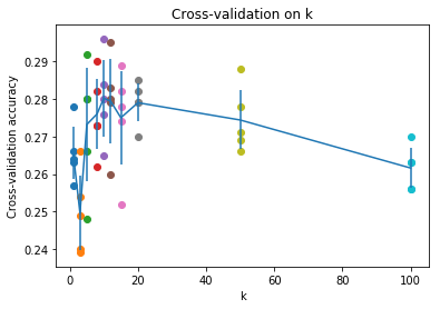
可以发现在此数据集下, 时效果最好。
现在可以跑一跑测试集了:
In[13]
# Based on the cross-validation results above, choose the best value for k,
# retrain the classifier using all the training data, and test it on the test
# data. You should be able to get above 28% accuracy on the test data.
best_k = 10

classifier = KNearestNeighbor()
classifier.train(X_train, y_train)
y_test_pred = classifier.predict(X_test, k=best_k)

# Compute and display the accuracy
num_correct = np.sum(y_test_pred == y_test)
accuracy = float(num_correct) / num_test
print('Got %d / %d correct => accuracy: %f' % (num_correct, num_test, accuracy))
Out[13]
Got 141 / 500 correct => accuracy: 0.282000最终我们获得了 的准确率。